RAPA Walkthrough

This tutorial is meant to cover multiple RAPA use cases, including starting from scratch or using a previous DataRobot project.

Overview

1. Initialize the DataRobot API

   • Save a pickled dictionary for DataRobot API Initialization

   • Use the pickled dictionary to initialize the DataRobot API

   • (Optional): Skip this if the DataRobot API is previously initialized

2. Submit data as a project to DataRobot

   • Create a submittable pandas dataframe

   • Submit the data using RAPA

   • (Optional): If parsimonious feature reduction is required on an existing project, it is possible to load the project instead of creating a new one.

3. Perform parsimonious feature reduction

[Link to the documentation]

import rapa
print(rapa.version.__version__)

0.1.0

1. Initialize DataRobot the API

import pickle
import os

On the DataRobot website , find the developer tools and retrieve an API key. Once you have a key, make sure to run the next block of code with your api key replacing the value in the dictionary. Here is a detailed article on DataRobot API keys.

Make sure to remove code creating the pickled dataframe and the pickled dataframe itself from any public documents, such as GitHub.

# save a pickled dictionary for datarobot api initialization
api_dict = {'tutorial':'APIKEYHERE'}
if 'data' in os.listdir('.'):
    print('data folder already exists, skipping folder creation...')
else:
    print('Creating data folder in the current directory.')
    os.mkdir('data')

if 'dr-tokens.pkl' in os.listdir('data'):
    print('dr-tokens.pkl already exists.')
else:
    with open('data/dr-tokens.pkl', 'wb') as handle:
        pickle.dump(api_dict, handle)

data folder already exists, skipping folder creation...
dr-tokens.pkl already exists.

# Use the pickled dictionary to initialize the DataRobot API
rapa.utils.initialize_dr_api('tutorial')

DataRobot API initiated with endpoint 'https://app.datarobot.com/api/v2'

The majority of this tutorial uses the DataRobot API, so if the API is not initialized, it will not run.

2. Submit data as a project to DataRobot

This tutorial uses the Breast cancer wisconsin (diagnostic) dataset as an easily accessible example set for rapa, as it easily loaded with sklearn.

This breast cancer dataset has 30 features extracted from digitized images of aspirated breast mass cells. A few features are the mean radius of the cells, the mean texture, mean perimater The target is whether the cells are from a malignant or benign tumor, with 1 indicating benign and 0 indicating malignant. There are 357 benign and 212 malignant samples, making 569 samples total.

from sklearn import datasets # data used in this tutorial
import pandas as pd # used for easy data management

# loads the dataset (as a dictionary)
breast_cancer_dataset = datasets.load_breast_cancer()

# puts features and targets from the dataset into a dataframe
breast_cancer_df = pd.DataFrame(data=breast_cancer_dataset['data'], columns=breast_cancer_dataset['feature_names'])
breast_cancer_df['benign'] = breast_cancer_dataset['target']
print(breast_cancer_df.shape)
breast_cancer_df.head()

(569, 31)

	mean radius	mean texture	mean perimeter	mean area	mean smoothness	mean compactness	mean concavity	mean concave points	mean symmetry	mean fractal dimension	...	worst texture	worst perimeter	worst area	worst smoothness	worst compactness	worst concavity	worst concave points	worst symmetry	worst fractal dimension	benign
0	17.99	10.38	122.80	1001.0	0.11840	0.27760	0.3001	0.14710	0.2419	0.07871	...	17.33	184.60	2019.0	0.1622	0.6656	0.7119	0.2654	0.4601	0.11890	0
1	20.57	17.77	132.90	1326.0	0.08474	0.07864	0.0869	0.07017	0.1812	0.05667	...	23.41	158.80	1956.0	0.1238	0.1866	0.2416	0.1860	0.2750	0.08902	0
2	19.69	21.25	130.00	1203.0	0.10960	0.15990	0.1974	0.12790	0.2069	0.05999	...	25.53	152.50	1709.0	0.1444	0.4245	0.4504	0.2430	0.3613	0.08758	0
3	11.42	20.38	77.58	386.1	0.14250	0.28390	0.2414	0.10520	0.2597	0.09744	...	26.50	98.87	567.7	0.2098	0.8663	0.6869	0.2575	0.6638	0.17300	0
4	20.29	14.34	135.10	1297.0	0.10030	0.13280	0.1980	0.10430	0.1809	0.05883	...	16.67	152.20	1575.0	0.1374	0.2050	0.4000	0.1625	0.2364	0.07678	0

5 rows × 31 columns

When using rapa to create a project on DataRobot, the number of features is reduced using on of the sklearn functions sklearn.feature_selection.f_classif, or sklearn.feature_selection.f_regress depending on the rapa instance that is called. In this tutorial’s case, the data is a binary classification problem, so we have to create an instance of the Project.Classification class.

As of now, rapa only supports classification and regression problems on DataRobot. Additionally, rapa has only been tested on tabular data.

# Creates a rapa classifcation object
bc_classification = rapa.Project.Classification()

# creates a datarobot submittable dataframe with cross validation folds stratified for the target (benign)
sub_df = bc_classification.create_submittable_dataframe(breast_cancer_df, target_name='benign')
print(sub_df.shape)
sub_df.head()

(569, 32)

	benign	partition	mean radius	mean texture	mean perimeter	mean area	mean smoothness	mean compactness	mean concavity	mean concave points	...	worst radius	worst texture	worst perimeter	worst area	worst smoothness	worst compactness	worst concavity	worst concave points	worst symmetry	worst fractal dimension
0	0	CV Fold 4	17.99	10.38	122.80	1001.0	0.11840	0.27760	0.3001	0.14710	...	25.38	17.33	184.60	2019.0	0.1622	0.6656	0.7119	0.2654	0.4601	0.11890
1	0	CV Fold 3	20.57	17.77	132.90	1326.0	0.08474	0.07864	0.0869	0.07017	...	24.99	23.41	158.80	1956.0	0.1238	0.1866	0.2416	0.1860	0.2750	0.08902
2	0	CV Fold 1	19.69	21.25	130.00	1203.0	0.10960	0.15990	0.1974	0.12790	...	23.57	25.53	152.50	1709.0	0.1444	0.4245	0.4504	0.2430	0.3613	0.08758
3	0	CV Fold 0	11.42	20.38	77.58	386.1	0.14250	0.28390	0.2414	0.10520	...	14.91	26.50	98.87	567.7	0.2098	0.8663	0.6869	0.2575	0.6638	0.17300
4	0	CV Fold 2	20.29	14.34	135.10	1297.0	0.10030	0.13280	0.1980	0.10430	...	22.54	16.67	152.20	1575.0	0.1374	0.2050	0.4000	0.1625	0.2364	0.07678

5 rows × 32 columns

# submits a project to datarobot using our dataframe, target, and project name.
project = bc_classification.submit_datarobot_project(input_data_df=sub_df, target_name='benign', project_name='TUTORIAL_breast_cancer')
project

Project(TUTORIAL_breast_cancer)

# if the project already exists, the `rapa.utils.find_project` function can be used to search for a project
project = rapa.utils.find_project("TUTORIAL_breast_cancer")
project

Project(TUTORIAL_breast_cancer)

3. Perform parsimonious feature reduction

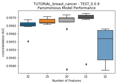
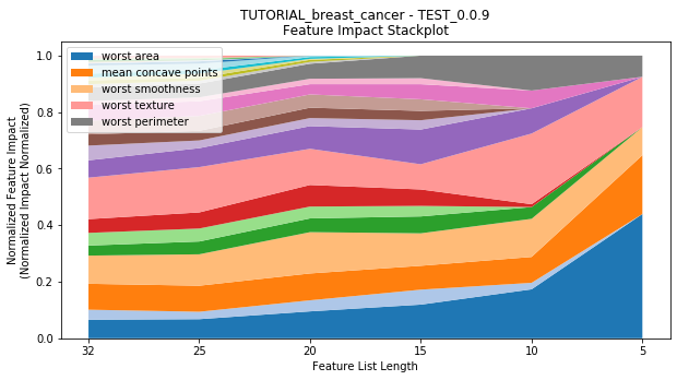
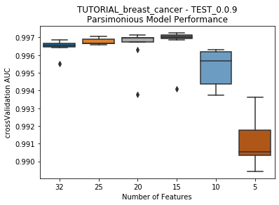
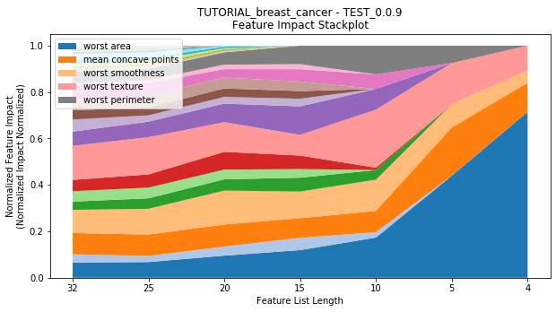
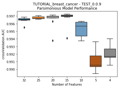
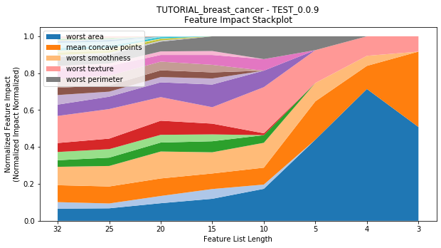
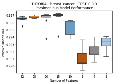
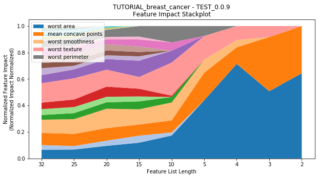
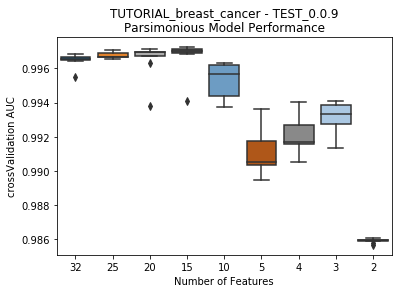
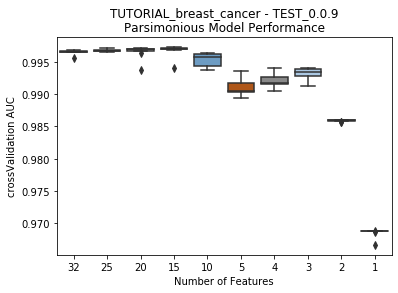
rapa’s main function is perform_parsimony. Requiring a feature_range and a project, this function recursively removes features by their relative feature impact scores across all models in a featurelist, creating a new featurelist and set of models with DataRobot each iteration.

• feature_range: a list of desired featurelist lengths as integers (Ex: [25, 20, 15, 10, 5, 4, 3, 2, 1]), or of desired featurelist sizes (Ex: [0.9, 0.7, 0.5, 0.3, 0.1]). This tells rapa how many features remain after each iteration of feature reduction.

• project: either a datarobot project, or a string of it’s id or name. rapa.utils.find_project can be used to find a project already existing in DataRobot, or submit_datarobot_project can be used to submit a new project.

• featurelist_prefix: provides datarobot with a prefix that will be used for all the featurelists created by the perform_parsimony function. If running rapa multiple times in one DataRobot project, make sure to change the featurelist_prefix each time to avoid confusion.

• starting_featurelist_name: the name of the featurelist you would like to start parsimonious reduction from. It defaults to ‘Informative Features’, but can be changed to any featurelist name that exists within the project.

• lives: number of times allowed for reducing the featurelist and obtaining a worse model. By default, ‘lives’ are off, and the entire ‘feature_range’ will be ran, but if supplied a number >= 0, then that is the number of ‘lives’ there are. (Ex: lives = 0, feature_range = [100, 90, 80, 50] RAPA finds that after making all the models for the length 80 featurelist, the ‘best’ model was created with the length 90 featurelist, so it stops and doesn’t make a featurelist of length 50.) This is similar to DataRobot’s Feature Importance Rank Ensembling for advanced feature selection (FIRE) package’s ‘lifes’.

• cv_average_mean_error_limit: limit of cross validation mean error to help avoid overfitting. By default, the limit is off, and the each ‘feature_range’ will be ran. Limit exists only if supplied a number >= 0.0.

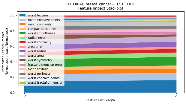
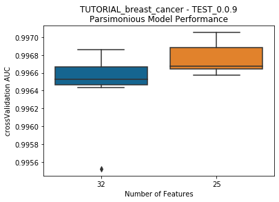
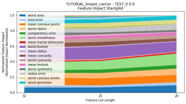
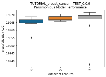
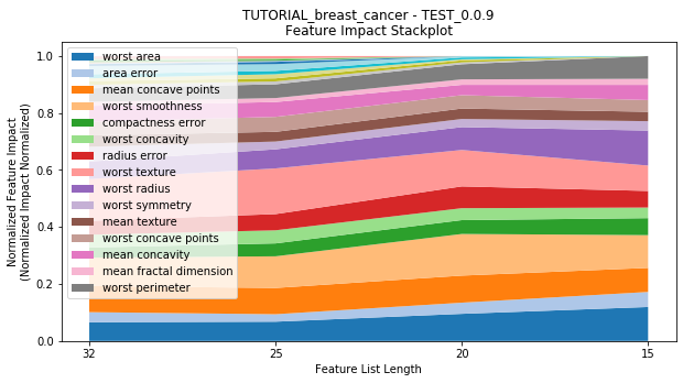
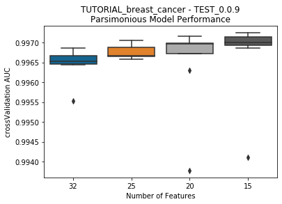
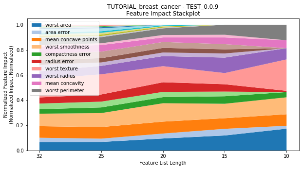
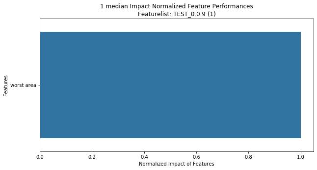
• to_graph: a list of keys choosing which graphs to produce. Current graphs are feature_performance and models. feature_performance graphs a stackplot of feature impacts across many featurelists, showing the change in impact over different featurelist lengths. models plots seaborn boxplots of some metric of accuracy for each featurelist length. These plots are created after each iteration.

Additional arguments and their effects can be found in the API documentation, or within the functions.

bc_classification.perform_parsimony(project=project,
                                    featurelist_prefix='TEST_' + str(rapa.version.__version__),
                                    starting_featurelist_name='Informative Features',
                                    feature_range=[25, 20, 15, 10, 5, 4, 3, 2, 1],
                                    lives=5,
                                    cv_average_mean_error_limit=.8,
                                    to_graph=['feature_performance', 'models'])

---------- Informative Features (30) ----------
Informative Features: Waiting for previous jobs to complete...
Previous job(s) remaining (0))
Informative Features: Waiting for feature impact...
Feature Impact job(s) remaining (0))
Feature Impact: (105.26s)
Graphing feature performance...

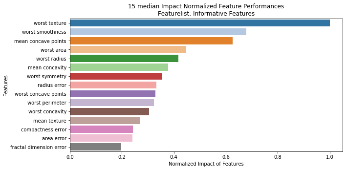
DataRobot job(s) remaining (0)
Project: TUTORIAL_breast_cancer | Featurelist Prefix: TEST_0.0.9 | Feature Range: [25, 20, 15, 10, 5, 4, 3, 2, 1]
Feature Importance Metric: median | Model Performance Metric: AUC
Lives: 5
CV Mean Error Limit: 0.8

---------- TEST_0.0.9 (25) ----------
Autopilot: 249.98s
Feature Impact job(s) remaining (0)
Feature Impact: 152.84s
Waiting for DataRobot: 10.71s

Performance Stackplot: 11.99s

Model Performance Boxplot: 0.94s
Checking lives: 5.58s
Lives left: 5 | Previous Model Best Score: 0.996862 | Current Best Model Score: 0.9970519999999999
Mean Error Limit: 1.10s
CV Error From the Mean: 0.005385306929239613 | CV Mean Error Limit: 0.8 | CV Model Performance Metric: AUC
---------- TEST_0.0.9 (20) ----------
Autopilot: 270.22s
Feature Impact job(s) remaining (0)
Feature Impact: 78.82s
Waiting for DataRobot: 10.67s

Performance Stackplot: 18.91s

Model Performance Boxplot: 1.17s
Checking lives: 11.45s
Lives left: 5 | Previous Model Best Score: 0.996862 | Current Best Model Score: 0.9970519999999999
Mean Error Limit: 1.19s
CV Error From the Mean: 0.005228428328360267 | CV Mean Error Limit: 0.8 | CV Model Performance Metric: AUC
---------- TEST_0.0.9 (15) ----------
Autopilot: 230.22s
Feature Impact job(s) remaining (0)
Feature Impact: 68.98s
Waiting for DataRobot: 10.58s

Performance Stackplot: 25.13s

Model Performance Boxplot: 1.35s
Checking lives: 16.93s
Lives left: 5 | Previous Model Best Score: 0.996862 | Current Best Model Score: 0.9970519999999999
Mean Error Limit: 1.44s
CV Error From the Mean: 0.005057377745942271 | CV Mean Error Limit: 0.8 | CV Model Performance Metric: AUC
---------- TEST_0.0.9 (10) ----------
Autopilot: 472.73s
Feature Impact job(s) remaining (0)
Feature Impact: 73.14s
Waiting for DataRobot: 10.95s

Performance Stackplot: 33.12s

Model Performance Boxplot: 1.70s
Current model performance: '0.997242'. Previous best model performance: '0.997242'
No change in the best model, so a life was lost.
Lives remaining: '4'
Checking lives: 23.74s
Lives left: 4 | Previous Model Best Score: 0.996862 | Current Best Model Score: 0.9970519999999999
Mean Error Limit: 1.21s
CV Error From the Mean: 0.004886720473612955 | CV Mean Error Limit: 0.8 | CV Model Performance Metric: AUC
---------- TEST_0.0.9 (5) ----------
Autopilot: 230.10s
Feature Impact job(s) remaining (0)
Feature Impact: 85.14s
Waiting for DataRobot: 10.64s

Performance Stackplot: 36.20s

Model Performance Boxplot: 2.38s
Current model performance: '0.997242'. Previous best model performance: '0.997242'
No change in the best model, so a life was lost.
Lives remaining: '3'
Checking lives: 27.89s
Lives left: 3 | Previous Model Best Score: 0.996862 | Current Best Model Score: 0.9970519999999999
Mean Error Limit: 1.43s
CV Error From the Mean: 0.009681340693827197 | CV Mean Error Limit: 0.8 | CV Model Performance Metric: AUC
---------- TEST_0.0.9 (4) ----------
Autopilot: 249.77s
Feature Impact job(s) remaining (0)
Feature Impact: 69.58s
Waiting for DataRobot: 10.57s

Performance Stackplot: 40.44s

Model Performance Boxplot: 2.22s
Current model performance: '0.997242'. Previous best model performance: '0.997242'
No change in the best model, so a life was lost.
Lives remaining: '2'
Checking lives: 32.98s
Lives left: 2 | Previous Model Best Score: 0.996862 | Current Best Model Score: 0.9970519999999999
Mean Error Limit: 1.81s
CV Error From the Mean: 0.00870168512405422 | CV Mean Error Limit: 0.8 | CV Model Performance Metric: AUC
---------- TEST_0.0.9 (3) ----------
Autopilot: 249.92s
Feature Impact job(s) remaining (0)
Feature Impact: 84.92s
Waiting for DataRobot: 10.33s

Performance Stackplot: 50.59s

Model Performance Boxplot: 2.77s
Current model performance: '0.997242'. Previous best model performance: '0.997242'
No change in the best model, so a life was lost.
Lives remaining: '1'
Checking lives: 40.55s
Lives left: 1 | Previous Model Best Score: 0.996862 | Current Best Model Score: 0.9970519999999999
Mean Error Limit: 1.25s
CV Error From the Mean: 0.005374831693523058 | CV Mean Error Limit: 0.8 | CV Model Performance Metric: AUC
---------- TEST_0.0.9 (2) ----------
Autopilot: 230.24s
Feature Impact job(s) remaining (0)
Feature Impact: 80.29s
Waiting for DataRobot: 10.61s

Performance Stackplot: 54.69s

Model Performance Boxplot: 2.78s
Current model performance: '0.997242'. Previous best model performance: '0.997242'
No change in the best model, so a life was lost.
Lives remaining: '0'
Checking lives: 43.40s
Lives left: 0 | Previous Model Best Score: 0.996862 | Current Best Model Score: 0.9970519999999999
Mean Error Limit: 1.06s
CV Error From the Mean: 0.007301264001862837 | CV Mean Error Limit: 0.8 | CV Model Performance Metric: AUC
---------- TEST_0.0.9 (1) ----------
Autopilot: 189.18s
Feature Impact job(s) remaining (0)
Feature Impact: 64.54s
Waiting for DataRobot: 10.16s

Performance Stackplot: 57.28s

Model Performance Boxplot: 2.91s
Current model performance: '0.997242'. Previous best model performance: '0.997242'
No change in the best model, so a life was lost.
Lives remaining: '-1'
Checking lives: 47.33s
Ran out of lives.
Best model: 'Model('Elastic-Net Classifier (L2 / Binomial Deviance)')'
Accuracy (AUC):'0.997242'

Finished Parsimony Analysis in 4211.28s.